started 26th July 2016 - completed 23rd September 2016
A modified version of the programmable unijunction transistor oscillator is found to be a passable source of random numbers.
Danneyelectronics blog [1] says that RC oscillators are good true random number generators (TRNG) due to their phase noise. Hmm I wonder how good a source of randomness the PUT oscillator is.
Quoting Wikipedia "phase noise is the frequency domain representation of rapid, short-term, random fluctuations in the phase of a waveform, caused by time domain instabilities (jitter). Generally speaking, radio frequency engineers speak of the phase noise of an oscillator, whereas digital system engineers work with the jitter of a clock."
I measured the time between output pulses using an Arduino Pro Mini based on the ATMega 328p, this has a timer capture register, so results should not be affected by interrupts. The clock is a crystal oscillator running at 16 MHz, which (see GPS) is likely to be accurate to better than a cycle per second.
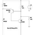
The PUT has an output which goes negative in around 1 μs, to match it to the ATMega 328p an inverting single transistor buffer is needed. The ATMega is set up to capture the time of the resulting positive edge. The point being that the pulses have fast rise times and there's not another lot of uncertainty around external comparators and their power supply voltages. The variations in period are visible on a 'scope.
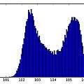
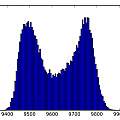
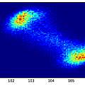
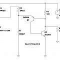
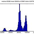
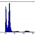
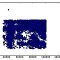
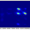
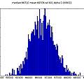
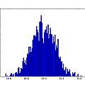
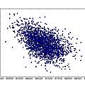
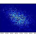
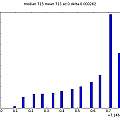
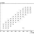
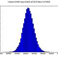
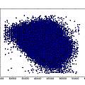
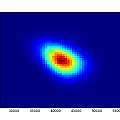
Graphics show PUT oscillator (I used a 5V supply and a 10nF capacitor, the output is taken from the junction of R1 and R2), histograms of output inverse time and time and a scatter plot of inverse time of cycle N against inverse time of cycle N+1.
The histograms do not look very random. As a crude test I plotted the inverse time of cycle N against that of cycle N+1. It seems that a short cycle is followed by a long one. I found a similar histogram in [4], which says it represents "deterministic jitter".
One possibility I could imagine is that a long cycle pulls down the power supply voltage a little and results in a following short cycle. I found no sign that this was going on, but the general idea that after a long cycle the circuit is in a state where the next cycle will be short seems plausible. In other words the circuit has to have a memory of the previous cycle.
After a while I noticed that the frequency of the oscillator happens to be nearly 100 Hz - the mains here is 50 Hz - allowing alternate half cycles to push and pull the oscillator frequency. I built the circuit on a typical solder-less breadboard; the connection between the collector of Q1 and the base of Q2 was three inches of insulated wire; replacing it with a much shorter connection made the double peaks less prominent whilst holding the wire between my fingers made the jitter worse. This point in the circuit has high impedance when the transistors are turned off.
Where does the characteristic shape of the histogram come from? Imagine that the oscillator is going a lot faster than the 50 Hz interference. Effectively an oscillation takes place with a fixed value of the interference. If that oscillation coincides with the maximum value of interference then the oscillation will have a minimum time, the other extreme of interference will give a maximum time. Given a sine wave (like the 50 Hz mains) for most of the time values are near one extreme or the other. The histogram is showing the probability distribution for a sine wave. The links [5] [6] [7] [8] confirm this idea.
Another way of putting this is that the oscillator is sampling the sine wave with the period of the oscillator being the value. Plotting the period of oscillation against time allows the interfering signal to be reconstructed - see later.
Looking at the PUT circuit above, if the voltage across C1 follows the usual RC equation (charging from a voltage Vs):
and the threshold at which the transistors turn on at is Vt, then the period will be:
For Vt/Vs=0.5 the ln is 0.7, for Vt/Vs=0.99 the ln is -4.6 and for Vt/Vs=0.999 the ln is -6.9 meaning that the period will not increase much even when Vt and Vs are within millivolts of one another.
There's a bit of messing about with Vbe - roughly the lowest voltage across C1 and the threshold is Vbe above the voltage at the junction of R1 and R2. As Vt approaches Vs the period gets longer.
The rate of change of voltage with respect to time is:
For large times the voltage does not change much.
The rate of change of period with respect to changes in the threshold voltage is:
When ` V_t ` approaches ` V_s ` period becomes sensitive to changes in ` V_t `.
All of which mean that a threshold far away from the supply voltage will be cut by a rapidly changing voltage and timings are relatively insensitive to changes in the threshold due to noise. Whilst a threshold close to Vs has the opposite behaviour.
For an oscillator with little jitter pick a threshold away from Vs, and for more jitter chose Vt close to Vs. One can vary Vs as easily as Vt.
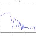
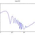
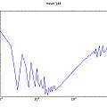
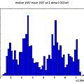
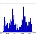
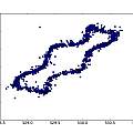
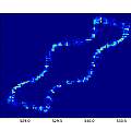
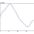
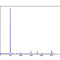
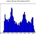
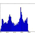
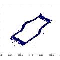
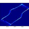
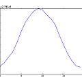
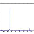
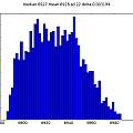
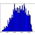
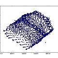
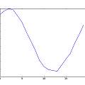
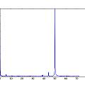
Three sets of graphics for Vs=5, 4 and 3V. Each set is histogram of time, inverse time, inverse timr N against N+1, inverse time N against N+1, reconstructed 50 Hz signal, and (jitter) frequency spectrum. For the reconstruction, the time duration of oscillation is being plotted against run time modulo 20 ms. For the frequency spectrum the time between pulses is used as a sample value and the time the pulse occurs at as the sample time. The last two are an approximation, reasonable if the oscillation period jitter is small compared to the period of oscillation. This time I used a 1nF capacitor.
Download 5V data
Download 4V data
Download 3V data
It is apparent there is 50 Hz interference. Again the circuit is on a solder-less bread board, but with no long wires. It's just very sensitive. As Vs decreases the time of oscillations increases whilst the spread in time increases showing the greater sensitivity to noise. Below 3V it gets difficult to adjust the voltage by hand, a little too low and oscillation stops.
Allan time
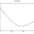
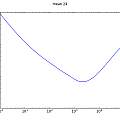
Seemingly [12] a good way to analyse data like this is to compute the "Allan deviation" [13] [14] [15] [16] [17] (square root of the Allan variance aka "two-sample variance") this compares the frequency of two samples rather than each sample with the mean (as for the standard deviation). The duration of the two samples compared is varied to give a (sigma - tau) plot. Graphs show the "overlapping Allan deviation" for the three voltages above.
The 50 Hz interference is apparent; see later for interpreting Allan deviation plots. The graphs were plotted using "allantools"[13].
[14] takes the point of view of how error varies with changing numbers of measurements. As the number of measurements increases the effects of noise cancel out. The Allan plot allows finding the number of measurements that minimises the error. In the Allan plot for 5V above the first dip is at around 10 samples, (at 529 Hz) 20 ms worth of oscillations, one mains cycle.
There are many ways of producing periodogram plots or finding weak cyclical signals in noise [18] [19].
Self adjusting PUT oscillator
Since the game is to produce randomness then an idea is for the circuit to use feedback to adjust Vs to be as close to Vt as possible whilst keeping oscillations going. If oscillations look like they are stopping the circuit can increase Vs and if the frequency is high it can reduce Vs. By this means one can ensure the voltage stays close to Vs for a long time and increase the sensitivity to noise.
The obvious implementation is to feed the output of the oscillator into a frequency to voltage converter and use the resulting voltage for Vs. However there is a simple addition to the PUT which gives the same effect which is shown below.
Graphics are the self adjusting PUT circuit, histogram of time, inverse time, inverse time of cycle N against cycle N+1.
LT Spice file of the circuit
Download data
The drop in frequency to 12 Hz from 144 Hz for Vs=3 V shows how effective the circuit is at adjusting Vs downwards whilst maintaining oscillation. Unfortunately this example boots the discussion into a different area - the jitter is no longer small - one cycle can take twice as long as the next. In addition the interference now is of a higher frequency than the oscillation. Another effect is visible, in the histogram of time durations there are bumps separated by roughly 20 ms, this is the effect of the 50 Hz noise on the long time when the voltage on C1 is close to Vt.
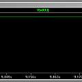
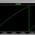
Compared to the standard PUT oscillator C1 will charge up to close to Vt almost as quickly but it will then spend a long time just below Vt. Graphics show the voltage across C1 for the self adjusting PUT oscillator and the standard version. For the former the simulation gives a gradient of around 6 mV per second - if it was true and if one could measure time to 1 μs then sensitivity would be in pico-Volts, down amongst thermal noise levels.
Graphics show the LT Spice results for the self adjusting PUT oscillator using the same values as above.
On the bright side, the 50 Hz interference has gone from these results (it's easy to simulate if desired) but they raise the problem of where all the noise is coming from - insignificant changes to the LT Spice model change the results, apparently then numerical noise.
Tin Man
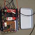
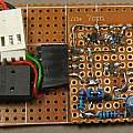
To get rid of the interference I built the PUT and self adjusting PUT oscillators in a tin box - also in the box were 3 AA NiMh batteries. Communication with the micro-controller was via an optical fibre cable. I used the TORX 178B and TOTX 179P receiver and transmitter and two metres of Toslink cable.
This did stop the interference, the results for the simple PUT oscillator effectively collapsed to a single frequency; variation in time was only as big as the 1/16 th μs resolution of the micro-controller.
Graphs show time between pulses, inverse time of N against N+1 and Allan deviation.
In contrast the self adjusting PUT oscillator produced a nice spread of times between pulses.
Graphs show time between pulses, inverse time of cycle N against N+1 and Allan deviation (overlapping, overlapping with gradients and modified with gradients).
Random results
Generating bits on the basis of the time between pulses being even or odd gave me a file of random data - this passed the rngtest (FIPS 140-2) and Dieharder 3.31.1 [25]. What happens with data from the breadboard PUT oscillator which has mains interference? Surprisingly the data fails rngtest but passes Dieharder.
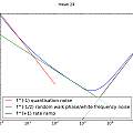
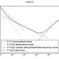
It is possible to derive information from the plot of Allan deviation by looking at the gradient (see graphic 5 in the previous set). It is common for low time values to be dominated by quantisation noise and high values by frequency drift. The best reference I found for interpreting plots is [27]. The modified Allan deviation allows distinguishing quantisation noise from white phase noise, this is shown in graphic 6 in the previous set.
From the graphics it appears that the self adjusting PUT oscillator sets off with white phase noise and ends with frequency drift. In the middle there is a range of random walk phase variation or white frequency noise.
Phase is the time integral of frequency. A random walk is the summation of independent, identically distributed random variables. It is possible to calculate the Allan deviation from the Power Spectral Density (PSD), but not the other way around, gradients only show what a given PSD would produce an Allan deviation looking like.
I worried if my use of Allan variance was correct. The discussions of Allan variance are presented from the point of view of someone with a 10 MHz oscillator and a frequency counter with a 1 second gate time. Every second they get a value for the frequency. They can compare one frequency value with the next. The point being the time between values is constant at one second, and the duration of comparisons can be varied in multiples of it.
Here the time between samples is not constant because it is the variable duration of the cycles. I am measuring the duration of single cycles not millions. The waveform is not sinusoidal and I can't measure the phase within a cycle, all I have are the times of events.
I came to the conclusion the results are valid. With Allantools there is a program which plots various types of noise ("noise color demo") allowing the Allan deviation results for each to be seen. For white noise it generates a series of random numbers and feeds them into the code for calculating the Allan deviation. There's no need for the complexity of equal sample times etc.
I also tried sampling my data with equal times (counting the number of cycles in every so long) and got the same result (phase random walk) although I lost the detail for times less than the sample time.
[29] says that the scatter plot of the form shown in the second graphic of the previous set is indicative of white phase noise.
Autocorrelation
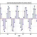
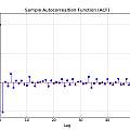
Ideally each cycle of the oscillator would be of random duration and independent of the preceding cycle. This would be white (frequency) noise, the corresponding phase would perform a random walk. Another test is to look at the auto-correlation of the series of times between pulses. The Ljung-Box test is a formal way of deciding if auto-correlations in time series are significant. Graphics show the auto-correlations for the 5V data above and self adjusting PUT oscillator (using code from [26])
As ever the 5V data have periodic interference and fail the Ljung Box test. The self adjusting PUT also fails. It is apparent there is a big correlation between neighbouring cycles (lag==1), for example a short period being followed by a long one. It puzzled me why the correlation is always around -0.5. Eventually I read in [28] ("5.5.4. The Lag 1 Autocorrelation") that this value is indicative of white phase noise - agreeing with the Allan deviation. (see Time Series for a derivation of the value).
Extracting every Nth data value (with N above 10) gives a series which does pass the test. So as the Allan deviation suggests, at long enough times there is randomness in frequency.
Calculating the 'phase', i.e. going back to the times of occurrence of pulses as opposed to the difference between them, also results in data which passes the test.
Humm
The modification to the PUT oscillator which makes it self adjust can be made to the other versions (see PUT2), some of those have desirable characteristics like working at higher frequencies.
A conclusion is that if a circuit has sensitivity to noise it is likely to also have sensitivity to external noise which may not be random.
Is there frequency locking? Yes where the period is greater than that of the interference, the capacitor voltage is just below the threshold for a long time, it is likely that a peak of the interference will push it over the threshold, so the period locks to a multiple of that of the interference.
In the other situation of oscillation period less than that of the interference, locking did not seem to occur. Pot twiddling it was difficult to make the oscillator work at exactly 50 Hz. For a lock to occur not only does the frequency have to be the same, but the phase has to be correct too, because period depends on interference phase. Half the interfering sine wave will work to increase errors in frequency (the other half decreases them). Perhaps this is a "phase anti-lock loop".
Software
Below is the code for measuring the oscillation period to run on the Arduino, Pro Mini, Uno etc or Pro Micro, Leonardo etc; different input pins have to be used depending on the processor. Secondly the Python code used to produce the graphs above, this can record from the USB port and save the data to a file, load a previously saved file or load data from LT Spice. In the first version of the Python code an apparently simple approach is horribly slow, the second version (suffixed 'fix') is much faster.
Download
- PhaseNoise01 Arduino sketch (8th September 2016)
- phasenoiseall00.py (8th September 2016)
- phasenoiseall00fix.py (8th September 2016)
References
- True Random Number Generators - Dannyelectronics
- Understanding and Characterizing Timing Jitter - Tektronix
- Noise in Relaxation Oscillators - A. A. Abidi and R. G. Meyer, IEEE JOURNAL OF SOLID-STATECIRCUITS,VOL. SC-18,NO. 6,DECEMBER 1983
- Basics of Phase Noise and Jitter - Asad Abidi, IEEE SSCS Chapter, Toronto: April 1, 2011
- Probability Density Function (pdf) of Sine Wave - Atif's blog
- Probability distribution for a noisy sine wave - stackexchange
- Probability Density Function pdf of Sine Wave - Google images
- Arcsine distribution - Wikipedia
- USING A 555 TIMER AND ADC AS A RANDOM SEED - Hackaday
- Arduino random numbers
- More Arduino random numbers
- Phase Noise- Enrico Rubiola
- Allantools - Anders E.E. Wallin
- Allan Deviation Primer - Phidgets
- The Allan Variance - David W. Allan
- AllanTools documentation
- AllanTools on Github
- Modeling Noisy Time Series: Least Squares Spectral Analysis - Charles H Martin, PhD
- Fast Lomb-Scargle Periodograms in Python - Jake Vanderplas
- Truth in Randomness - Microsemi
- Recovering Signals from Unevenly Sampled Data - Joseph Long
- APPLICATION NOTE 3359 Clock (CLK) Jitter and Phase Noise Conversion - Maxim
- High-Speed capture mit ATmega Timer - Michael Dreher
- Random sampling and reconstruction of spectra - Elias Masry
- Dieharder: A Random Number Test Suite - Robert G. Brown Dirk Eddelbuettel David Bauer
- Ljung-Box Test - Python Pattern Recognition
- IEEE Standard Specification Format Guide and Test Procedure for Single-Axis Interferometric Fiber Optic Gyros - IEEE Std 952-1997
- NIST Special Publication 1065 Handbook of Frequency Stability Analysis - W.J. Riley
- Use of the Autocorrelation Function for Frequency Stability Analysis - W.J. Riley
